人工智慧/機器學習/資料探勘正夯,剛好tidymodels套件組的官網上線了,順勢介紹由caret套件的開發者Max Kuhn所帶領開發的全新建模架構tidymodels並完成此篇教學文章。如同套件名稱,tidymodels套件組的撰寫邏輯和方法與tidyverse套件組合相同,若熟悉dplyr、ggplot等套件應該蠻好上手
第一次使用前一樣要先安裝
install.packages("tidymodels")安裝後即可載入
library(tidymodels)載入建模過程需要的其他套件,themis套件是做unser sampling或over sampling前處理會用到,vip套件則是用在輸出隨機森林Random Forest模型中各變數的重要性。
library(themis)
library(vip)
建模範例資料以及刪除遺漏值
這邊使用mlbench套件中的PimaIndiansDiabetes2資料集,該資料集的Outcome為是否有糖尿病diabetes,變數我就不一一介紹了,可輸入?PimaIndiansDiabetes2查看。
library(mlbench)
data("PimaIndiansDiabetes2")
資料載入後,習慣先看一下各資料的型態跟資料筆數,可以發現有不少NA值
glimpse(PimaIndiansDiabetes2)## Rows: 768
## Columns: 9
## $ pregnant <dbl> 6, 1, 8, 1, 0, 5, 3, 10, 2, 8, 4, 10, 10, 1, 5, 7, 0, 7, 1...
## $ glucose <dbl> 148, 85, 183, 89, 137, 116, 78, 115, 197, 125, 110, 168, 1...
## $ pressure <dbl> 72, 66, 64, 66, 40, 74, 50, NA, 70, 96, 92, 74, 80, 60, 72...
## $ triceps <dbl> 35, 29, NA, 23, 35, NA, 32, NA, 45, NA, NA, NA, NA, 23, 19...
## $ insulin <dbl> NA, NA, NA, 94, 168, NA, 88, NA, 543, NA, NA, NA, NA, 846,...
## $ mass <dbl> 33.6, 26.6, 23.3, 28.1, 43.1, 25.6, 31.0, 35.3, 30.5, NA, ...
## $ pedigree <dbl> 0.627, 0.351, 0.672, 0.167, 2.288, 0.201, 0.248, 0.134, 0....
## $ age <dbl> 50, 31, 32, 21, 33, 30, 26, 29, 53, 54, 30, 34, 57, 59, 51...
## $ diabetes <fct> pos, neg, pos, neg, pos, neg, pos, neg, pos, pos, neg, pos...在刪除不全的資料前,先看一下有糖尿病diabetes跟沒有糖尿病的人數與比例,大概是65:35,有些不平均不過還行。
PimaIndiansDiabetes2 %>%
  count(diabetes) %>%
  mutate(prop = n/sum(n))
## # A tibble: 2 x 3
## diabetes n prop
## <fct> <int> <dbl>
## 1 neg 500 0.651
## 2 pos 268 0.349通常有NA的資料不太會留,因為某些演算法不能用有NA的資料建模,雖然tidymodels有其他方法可以將NA資料去除,但為了後續基礎統計方便,如果要刪NA我還是習慣先全數刪除。
PimaIndiansDiabetes2<-
  PimaIndiansDiabetes2 %>%
  filter(complete.cases(PimaIndiansDiabetes2))
刪除NA後資料筆數有些微改變,但大概還是6x:3x的比例
PimaIndiansDiabetes2 %>%
  count(diabetes) %>%
  mutate(prop = n/sum(n))
## # A tibble: 2 x 3
## diabetes n prop
## <fct> <int> <dbl>
## 1 neg 262 0.668
## 2 pos 130 0.332完成初步資料排除後,就可以開始基礎統計分析與建模,基礎統計分析可看其他文章,這篇著重在建模。
訓練/調整與驗證模型效能策略
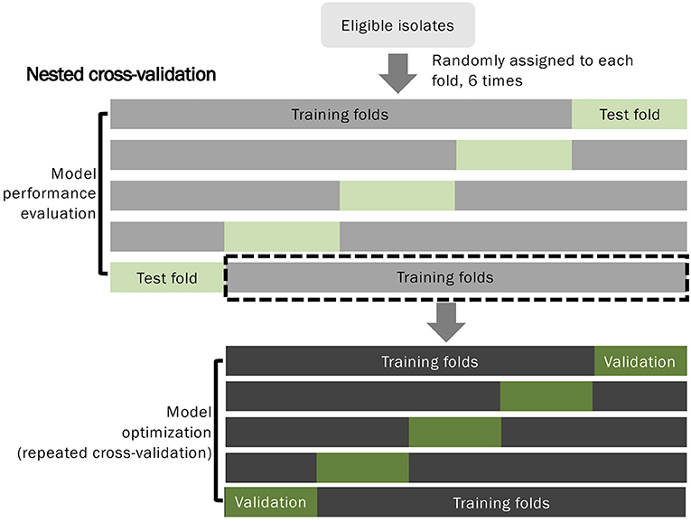
JAMA在2019年刊登一篇有趣的文章,名稱為How to Read Articles That Use Machine Learning - Users’ Guides to the Medical Literature 下載,內文中有提到在機器學習時代,如何建立與預測模型,跟之前又有什麼不同,並用下圖來解釋差異

在所謂的“非”機器學習模型(圖上半部),通常可分訓練組與測試組,在作者定義為Development set和Validation set,重要的概念是訓練模型時,一定要記得先把測試組資料分出來,不可以用到這部分資料來訓練模型,最後才能得到真實的預測結果 (完全沒偷看答案的意思)。
在圖下半部,作者將此法命名為3-step process,主要差異是在訓練模型時多了一組參數調整資料集,原因是因為在多種機器學習模型中,有可調整的參數,在圖中稱為Hyperparameters,為了讓調整效果更好,會將訓練組再切分成小組,用來決定最佳參數,決定好以後,才用所有訓練組資料搭配最佳參數訓練模型,最後再用測試組做測試。
以下用邏輯迴歸歸Logistic Regression示範此圖上半部不調參數的作法,以及用隨機森林Random Forest示範此圖下半部需要調整參數的作法。
訓練組、測試組資料分割
不管要不要調參數,都需要分割訓練組與測試組,因此在進入兩個範例前,先將訓練組與測試組切好。
用initial_split()函數將資料分成訓練組與測試組,第一個參數放資料,第二個參數prop放訓練組測試組比例,第三個參數strata放分組抽樣依據。需要設定分組抽樣依據是因為若是整批資料隨機抽樣,很有可能在測試組或是訓練組會少一整個組別的資料(剛好都沒抽到的意思),所以就分組,個別抽某個比例的人當訓練組,剩下的就當測試組。切割完後,用training()和testing()函數將訓練組測試組正式分開。
這邊要特別注意的是,因為initial_split()函數有隨機的概念,為了讓每次的實驗結果相同,我們會在有隨機事件前設定seed,作為隨機的依據,讓隨機每次都一樣,才不會每次跑都是不一樣的結果,這樣就無法產生可重複的實驗結果。
set.seed(123)
splits<- initial_split(PimaIndiansDiabetes2,
                       prop=(3/4),
                       strata = diabetes)
DM_train<- training(splits)
DM_test<- testing(splits)
分組完後,查看訓練組的生病比例
DM_train %>%
  count(diabetes) %>%
  mutate(prop = n/sum(n))
## # A tibble: 2 x 3
## diabetes n prop
## <fct> <int> <dbl>
## 1 neg 197 0.668
## 2 pos 98 0.332查看測試組的生病比例
DM_test %>%
  count(diabetes) %>%
  mutate(prop = n/sum(n))
## # A tibble: 2 x 3
## diabetes n prop
## <fct> <int> <dbl>
## 1 neg 65 0.670
## 2 pos 32 0.330建立資料前處理“食譜”
資料前處理也是建立兩種模型都必須經歷的方法,因此提到最前方說明,前處理有很多方法,包括將類別變項轉為虛擬變項(dummy variables),數值變項取log,數值變項正規化,以及日期資料處理等。
首先使用recipe()函數,設定模型訓練公式diabetes ~ .以及訓練用資料DM_train,要注意這邊只能用訓練組資料,不能用全部的資料。公式的意思是用~前方的diabetes當成outcome (想要預測的值),~後方的.代表其他所有剩下的欄位都當成predictors (又稱variables 或是 features,為預測基礎)。
完成模型公式與資料設定後,就開始逐一加上想要做的資料前處理方法,在這邊列舉幾項我認為以此案例可能需要做的前處理
step_naomit(everything(), skip = TRUE)如果沒有在一開始將NA資料刪掉,通常要去除NA值step_rose(diabetes)其實這個資料有病沒病的人沒差太多,只是呈現一下可以在此步驟設定oversampleing或是undersampling,這邊是指使用ROSE作為oversampling的演算法step_dummy(all_nominal(), -all_outcomes())將所有的類別變項轉成虛擬變項,除了Outcome以外step_zv(all_predictors())若有變項都是一樣的值,刪掉。舉例來說,若是整個資料都是女性,那性別欄位就不用拿來當作features了step_normalize(all_predictors())將所有數值變項正規化
還有很多其他的前處理方法,可以參考recipe()函數的說明文件
gen_recipe <-
  recipe(diabetes ~ ., data = DM_train) %>%
  step_dummy(all_nominal(), -all_outcomes()) %>%
  step_zv(all_predictors()) %>%
  step_normalize(all_predictors())
summary(gen_recipe)
## # A tibble: 9 x 4
## variable type role source
## <chr> <chr> <chr> <chr>
## 1 pregnant numeric predictor original
## 2 glucose numeric predictor original
## 3 pressure numeric predictor original
## 4 triceps numeric predictor original
## 5 insulin numeric predictor original
## 6 mass numeric predictor original
## 7 pedigree numeric predictor original
## 8 age numeric predictor original
## 9 diabetes nominal outcome original邏輯迴歸Logistic Regression模型建立與效能評估範例
Step 1 設定用邏輯迴建立模型
這邊以邏輯迴歸為例,用logistic_reg()函數與set_engine("glm")設定模型建立演算法為邏輯迴歸
lr_mod <-
  logistic_reg() %>%
  set_engine("glm")
Step 2 設定建模流程workflow
workflow將建模 (model)與資料前處理方法 (recipe)串成單一工作流程workflow
lr_wflow <-
  workflow() %>%
  add_model(lr_mod) %>%
  add_recipe(gen_recipe)
lr_wflow
## == Workflow ==============================================================================================
## Preprocessor: Recipe
## Model: logistic_reg()
##
## -- Preprocessor ------------------------------------------------------------------------------------------
## 3 Recipe Steps
##
## * step_dummy()
## * step_zv()
## * step_normalize()
##
## -- Model -------------------------------------------------------------------------------------------------
## Logistic Regression Model Specification (classification)
##
## Computational engine: glmStep 3 訓練模型
使用剛剛串起來的工作流程,加上fit()函數,完成建模,並用pull_workflow_fit()與tidy()呈現建模結果,注意這裡也是只能用訓練組資料DM_train
lr_fit <-
  lr_wflow %>%
  fit(data=DM_train)

lr_fit %>%
  pull_workflow_fit() %>%
  tidy()
## # A tibble: 9 x 5
## term estimate std.error statistic p.value
## <chr> <dbl> <dbl> <dbl> <dbl>
## 1 (Intercept) -0.940 0.158 -5.97 0.00000000244
## 2 pregnant 0.223 0.197 1.13 0.257
## 3 glucose 1.07 0.195 5.49 0.0000000405
## 4 pressure -0.116 0.162 -0.715 0.474
## 5 triceps -0.0127 0.202 -0.0629 0.950
## 6 insulin -0.0926 0.175 -0.530 0.596
## 7 mass 0.500 0.211 2.37 0.0179
## 8 pedigree 0.309 0.166 1.86 0.0631
## 9 age 0.392 0.208 1.88 0.0601Step 4 使用模型與測試組資料驗證模型效能
使用predict()函數,用剛剛訓練出來的模型lr_fit以及一開始分出的測試組DM_test產生預測結果,注意這邊要用測試組資料
lr_pred <- lr_fit %>%
  predict(DM_test)
lr_pred
## # A tibble: 97 x 1
## .pred_class
## <fct>
## 1 pos
## 2 neg
## 3 neg
## 4 pos
## 5 pos
## 6 pos
## 7 neg
## 8 neg
## 9 neg
## 10 neg
## # ... with 87 more rows將預測結果與答案結合
lr_pred <- lr_fit %>%
  predict(DM_test) %>%
  bind_cols(DM_test %>% select(diabetes))
lr_pred
## # A tibble: 97 x 2
## .pred_class diabetes
## <fct> <fct>
## 1 pos pos
## 2 neg pos
## 3 neg neg
## 4 pos pos
## 5 pos pos
## 6 pos pos
## 7 neg neg
## 8 neg neg
## 9 neg neg
## 10 neg neg
## # ... with 87 more rows使用accuracy()函數,輸入預測結果與真實答案計算正確率
lr_pred %>%
  accuracy(truth = diabetes,
          .pred_class)
## # A tibble: 1 x 3
## .metric .estimator .estimate
## <chr> <chr> <dbl>
## 1 accuracy binary 0.814但很多時候我們需要Area under the ROC curve,此時我們需要的不是直接pos或neg的結果,我們需要的是連續性的預測數值,這邊可將predict()函數的type參數設定為prob,即回傳各組預測值
lr_pred <- lr_fit %>%
  predict(DM_test,
          type = "prob")%>%
  bind_cols(DM_test %>% select(diabetes))
lr_pred
## # A tibble: 97 x 3
## .pred_neg .pred_pos diabetes
## <dbl> <dbl> <fct>
## 1 0.180 0.820 pos
## 2 0.648 0.352 pos
## 3 0.850 0.150 neg
## 4 0.0683 0.932 pos
## 5 0.125 0.875 pos
## 6 0.126 0.874 pos
## 7 0.854 0.146 neg
## 8 0.963 0.0366 neg
## 9 0.824 0.176 neg
## 10 0.733 0.267 neg
## # ... with 87 more rows得到各組預測值後,可用roc_curve()畫ROC curve
lr_pred %>%
  roc_curve(truth = diabetes,
            .pred_pos) %>%
  autoplot()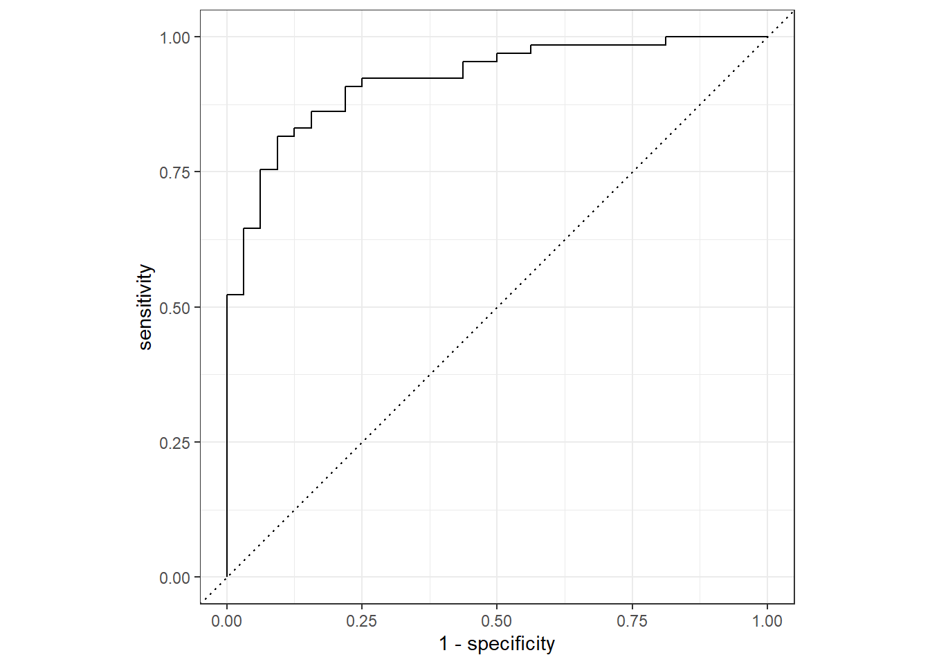
當然也能用roc_auc()算Area under the ROC curve
lr_pred %>%
  roc_auc(truth = diabetes,
          .pred_pos)
## # A tibble: 1 x 3
## .metric .estimator .estimate
## <chr> <chr> <dbl>
## 1 roc_auc binary 0.921以上就是使用邏輯迴歸建立模型與效能測試流程,可以發現完全沒有調整任何參數,因基本邏輯迴歸不用調參數。
隨機森林Random Forest模型建立、參數調整與效能評估範例
Step 1 設定平行處理
因為模型參數調整需要一直不斷建立模型與測試,所以設定平行處理會快一些,tidymodels套組支援平行處理,細節可參考官方文件
all_cores <- parallel::detectCores(logical = FALSE)
library(doParallel)
cl <- makePSOCKcluster(all_cores)
registerDoParallel(cl)
Step 2 設定用隨機森林建立模型以及要調整的參數
這邊以隨機森林為例,用rand_forest()函數與set_engine("ranger")設定模型建立演算法為基於ranger套件的隨機森林演算法,因為隨機森林有迴歸版與分類版,因此使用set_mode("classification")設定我們要用分類演算法。
在隨機森林rand_forest()函數中,可設定幾個參數,說明如下:
- mtry: 在切割節點時,隨機抽取n個特徵,並從中選最適合的特徵當作節點
- min_n: 每個節點的最小資料數,如果設為10,當該節點的資料剩十筆或更少時,就不會再切割
- trees: 建模要用幾棵樹
在這個範例中,我將要建幾棵樹設定為1000,其他兩個參數則是想用交叉驗證法(Cross Validation)來調整,因此將想調的參數值設為tune(),表示這些參數要調,不想在現階段指定。
rf_mod <-
  rand_forest(mtry = tune(), min_n = tune(),
              trees = 1000) %>%
  set_engine("ranger") %>%
  set_mode("classification")

rf_mod
## Random Forest Model Specification (classification)
##
## Main Arguments:
## mtry = tune()
## trees = 1000
## min_n = tune()
##
## Computational engine: rangerStep 3 設定建模流程workflow
建模流程同邏輯迴歸,將模型與資料前處理方法串接成一個工作流程
rf_wflow <- workflow() %>%
  add_model(rf_mod) %>%
  add_recipe(gen_recipe)
Step 4 參數調整組資料分割
剛剛有提到我想要調整的參數為mtry以及min_n,調整的方法為交叉驗證法(Cross Validation),這邊用tidymodels官網的圖來說明架構

在圖中,首先將所有資料分成測試組訓練組,也就是本篇文章一開始做的切割,為了調整參數,我們會再切訓練組的資料,做為測試各參數效能的調整訓練以及調整測試。
切割參數調整組有很多種方法,可以用bootstrap法隨機抽,也可使用這邊的交叉驗證範例,交叉驗證的概念如下圖的下半部
圖片下半部為5-fold Cross Validation的示意圖,可以看到每份資料都會被拿來當作調整訓練以及調整測試組,經過幾次測試後,用調整測試組的效能來決定一組最佳參數。
這邊我們使用10-fold Cross Validation為例,先用vfold_cv()函數,設定分割基準為訓練組,要分10份v=10,分割時一樣要注意糖尿病的比例不能差太多
set.seed(345)
folds <- vfold_cv(DM_train, v = 10,
                  strata = diabetes)
folds
## # 10-fold cross-validation using stratification
## # A tibble: 10 x 2
## splits id
## <named list> <chr>
## 1 <split [265/30]> Fold01
## 2 <split [265/30]> Fold02
## 3 <split [265/30]> Fold03
## 4 <split [265/30]> Fold04
## 5 <split [265/30]> Fold05
## 6 <split [265/30]> Fold06
## 7 <split [265/30]> Fold07
## 8 <split [266/29]> Fold08
## 9 <split [267/28]> Fold09
## 10 <split [267/28]> Fold10Step 5 調整參數
完成分割後,可將之前的建模流程串接至tune_grid()函數,這個函數可以設定參數調整的方法,首先是調整要用的參數調整組資料resamples = folds,要測試幾組參數grid = 50,測試時要用什麼效能評估方式,這邊設定為Area under the ROC curve metrics = metric_set(roc_auc)。另外參數的產生也有隨機的成分,需要set.seed()。因為要重複訓練測試多次,因此這程式碼執行會需要一些時間。
set.seed(345)
rf_res <-
  rf_wflow %>%
  tune_grid(
    resamples = folds,
    grid = 50,
    metrics = metric_set(roc_auc),
    control=control_resamples(save_pred = TRUE)
)執行完後,可用collect_metrics()查看各參數效能
rf_res %>%
  collect_metrics()
## # A tibble: 49 x 7
## mtry min_n .metric .estimator mean n std_err
## <int> <int> <chr> <chr> <dbl> <int> <dbl>
## 1 1 15 roc_auc binary 0.800 10 0.0246
## 2 1 24 roc_auc binary 0.804 10 0.0270
## 3 1 31 roc_auc binary 0.809 10 0.0258
## 4 1 35 roc_auc binary 0.808 10 0.0258
## 5 2 2 roc_auc binary 0.800 10 0.0231
## 6 2 8 roc_auc binary 0.803 10 0.0229
## 7 2 12 roc_auc binary 0.804 10 0.0224
## 8 2 19 roc_auc binary 0.807 10 0.0228
## 9 2 24 roc_auc binary 0.809 10 0.0228
## 10 2 33 roc_auc binary 0.810 10 0.0243
## # ... with 39 more rows也可畫個圖呈現參數調整對效能的影響,由圖可知在這個範例中min_n越大效能越好
rf_res %>%
  collect_metrics() %>%
  mutate(mtry = factor(mtry)) %>%
  ggplot(aes(min_n, mean, color = mtry)) +
  geom_line(size=1) +
scale_x_log10(labels = scales::label_number()) 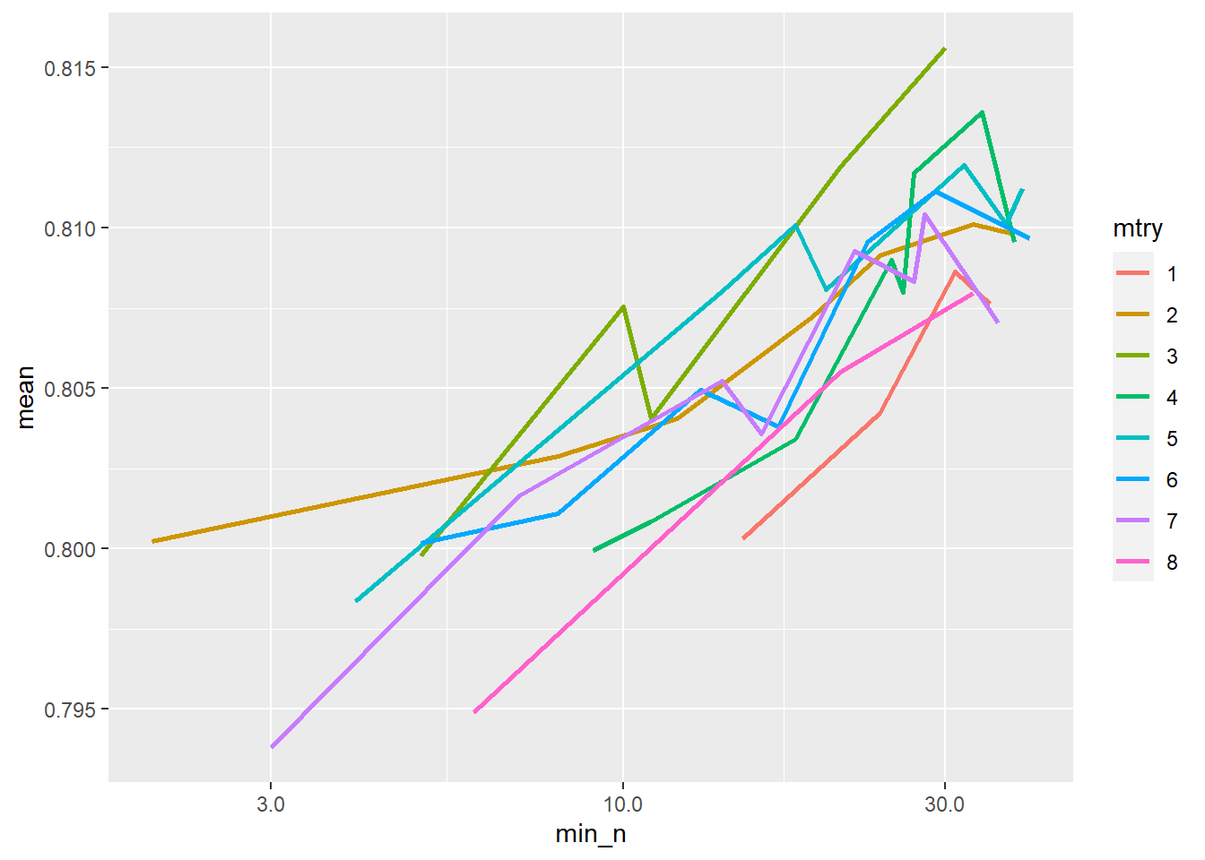
搭配show_best()函數可呈現Area under the ROC curve最優的幾組參數
rf_res %>%
  show_best("roc_auc")
## # A tibble: 5 x 7
## mtry min_n .metric .estimator mean n std_err
## <int> <int> <chr> <chr> <dbl> <int> <dbl>
## 1 3 30 roc_auc binary 0.816 10 0.0223
## 2 4 34 roc_auc binary 0.814 10 0.0227
## 3 5 32 roc_auc binary 0.812 10 0.0208
## 4 3 21 roc_auc binary 0.812 10 0.0205
## 5 4 27 roc_auc binary 0.812 10 0.0222Step 6 使用最佳參數與訓練組資料建立最終模型
在完成參數調整後,我們會使用最佳參數(意即Area under the ROC curve最高的一組參數)來建立最終模型,用select_best()函數可選出最好的一組參數best_rf
best_rf <- rf_res %>%
  select_best("roc_auc")
best_rf
## # A tibble: 1 x 2
## mtry min_n
## <int> <int>
## 1 3 30為了將參數節合至原有的建模流程,可用finalize_workflow()函數輸入剛剛選出的最佳參數best_rf,建立一個最終建模流程
final_wflow <-
  rf_wflow %>%
  finalize_workflow(best_rf)

final_wflow
## == Workflow ==============================================================================================
## Preprocessor: Recipe
## Model: rand_forest()
##
## -- Preprocessor ------------------------------------------------------------------------------------------
## 3 Recipe Steps
##
## * step_dummy()
## * step_zv()
## * step_normalize()
##
## -- Model -------------------------------------------------------------------------------------------------
## Random Forest Model Specification (classification)
##
## Main Arguments:
## mtry = 3
## trees = 1000
## min_n = 30
##
## Computational engine: ranger最終建模流程建立後,即可用fit()建模,注意這邊用的是完整的訓練資料DM_train
final_rf_model <-
  final_wflow %>%
  fit(data = DM_train)

final_rf_model
## == Workflow [trained] ====================================================================================
## Preprocessor: Recipe
## Model: rand_forest()
##
## -- Preprocessor ------------------------------------------------------------------------------------------
## 3 Recipe Steps
##
## * step_dummy()
## * step_zv()
## * step_normalize()
##
## -- Model -------------------------------------------------------------------------------------------------
## Ranger result
##
## Call:
## ranger::ranger(formula = formula, data = data, mtry = ~3L, num.trees = ~1000, min.node.size = ~30L, num.threads = 1, verbose = FALSE, seed = sample.int(10^5, 1), probability = TRUE)
##
## Type: Probability estimation
## Number of trees: 1000
## Sample size: 295
## Number of independent variables: 8
## Mtry: 3
## Target node size: 30
## Variable importance mode: none
## Splitrule: gini
## OOB prediction error (Brier s.): 0.1573813Step 7 用測試組資料驗證最終模型效能
使用predict()函數,用剛剛訓練出來的模型final_rf_model以及一開始分出的測試組DM_test產生預測結果,注意這邊要用測試組資料
rf_pred <- final_rf_model %>%
  predict(DM_test)
rf_pred
## # A tibble: 97 x 1
## .pred_class
## <fct>
## 1 pos
## 2 neg
## 3 neg
## 4 pos
## 5 pos
## 6 pos
## 7 neg
## 8 neg
## 9 neg
## 10 neg
## # ... with 87 more rows將預測結果與答案結合
rf_pred <- final_rf_model %>%
  predict(DM_test) %>%
  bind_cols(DM_test %>% select(diabetes))
rf_pred
## # A tibble: 97 x 2
## .pred_class diabetes
## <fct> <fct>
## 1 pos pos
## 2 neg pos
## 3 neg neg
## 4 pos pos
## 5 pos pos
## 6 pos pos
## 7 neg neg
## 8 neg neg
## 9 neg neg
## 10 neg neg
## # ... with 87 more rows使用預測結果與真實答案計算正確率
rf_pred %>%
  accuracy(truth = diabetes,
          .pred_class)
## # A tibble: 1 x 3
## .metric .estimator .estimate
## <chr> <chr> <dbl>
## 1 accuracy binary 0.804但很多時候我們需要Area under the ROC curve,此時我們需要的不是直接pos或neg的結果,我們需要的是連續性的預測數值,這邊可將predict()函數的type參數設定為prob,即回傳各組預測值
rf_pred <- final_rf_model %>%
  predict(DM_test,
          type = "prob")%>%
  bind_cols(DM_test %>% select(diabetes))
rf_pred
## # A tibble: 97 x 3
## .pred_neg .pred_pos diabetes
## <dbl> <dbl> <fct>
## 1 0.361 0.639 pos
## 2 0.526 0.474 pos
## 3 0.662 0.338 neg
## 4 0.177 0.823 pos
## 5 0.130 0.870 pos
## 6 0.191 0.809 pos
## 7 0.860 0.140 neg
## 8 0.956 0.0441 neg
## 9 0.793 0.207 neg
## 10 0.638 0.362 neg
## # ... with 87 more rows得到各組預測值後,可用roc_curve()畫ROC curve
rf_pred %>%
  roc_curve(truth = diabetes,
            .pred_pos) %>%
  autoplot()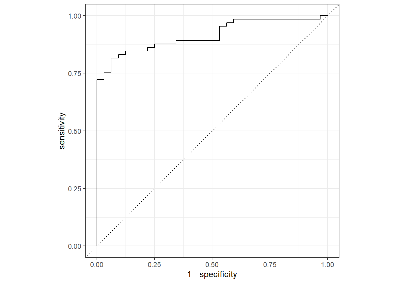
當然也能用roc_auc()算Area under the ROC curve
rf_pred %>%
  roc_auc(truth = diabetes,
          .pred_pos)
## # A tibble: 1 x 3
## .metric .estimator .estimate
## <chr> <chr> <dbl>
## 1 roc_auc binary 0.914以上就是使用隨機森林建立模型、調整參數以及與效能測試流程,多了使用交叉驗證法調整參數的步驟。